The Mandelbrot Set

The Mandelbrot set is a subset of the complex numbers \(\mathbb{C}\) obtained by the following iteration formula:

\[\begin{align*} z_0 &= c \\ z_{n+1} &= z_n^2 + z_0 \end{align*}\]

All variables denote complex numbers or, which is essentially the same, points on the complex number plane. The number \(c \in \mathbb{C}\) is called the starting point. If the iteration scheme is successively applied to the starting point, a sequence \((c_n)\) is obtained, which is called the orbit of \(c\).

For different starting points the orbit unfolds very differently. For some, the orbit elements quickly become larger and larger. For others, the orbit elements remain bounded for a long time before escaping. In some cases, the orbit elemenets do not escape at all. The starting points of these orbits are of particular interest. Together they form the Mandelbrot set \(M\):

\[\begin{align*} M := \{ c \text{ in } \mathbb{C} \;\; | \;\; ( |c_n| ) \not\rightarrow \infty \} \end{align*}\]

Expressed in words, the Mandelbrot set is the set of all complex numbers with a non-escaping orbit.

The fractal images we usually associate with the notion of the Mandelbrot set are certain visualizations of \(M\). To generate such an image, a certain section of the complex number plane is superimposed with a pixel grid. Each pixel then corresponds to a complex number \(c = x + y\,\text{i}\) for which the orbit \((c_n)\) is computed. In the next step, a coloring function is applied to \((c_n)\) which determines the color value.

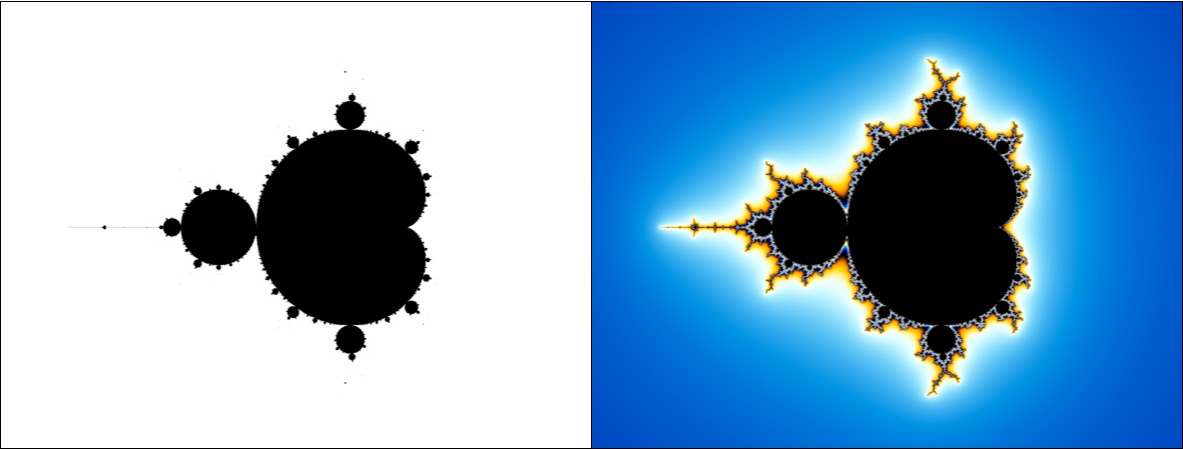
The image below shows two different colorizations of the Mandelbrot set. In the left image, all points inside the Mandelbrot set are colored black, all others are colored white. In the right image, a more complicated coloring function is utilized which derives the color value for all point outside the Mandelbrot set by analyzing the growth-rate of \((c_n)\) at the point where the sequence escapes.

If the Mandelbrot algorithm is implemented in a naive way by representing a complex number by two floating point numbers of type float or double a boundary is quickly reached. Beyond a certain zoom level, these data types are no longer capable of representing the numerical values with sufficient accuracy. From a theoretical point of view, this problem can be circumvented by utilizing multi-precision libraries that are capable of representing floating-point numbers in arbitrary precision. In practice, however, this is not a viable approach, since such libraries operate several orders of magnitude slower than the data types that are native to the CPU. Furthermore, with increasing zoom levels, an increasingly longer initial segment of the orbit must be calculated to obtain a reliable estimate about its convergence or divergence. This was the situation for many years. It seemed as if very deep views into the Mandelbrot set would remain practically impossible.

In 2013, the situation changed virtually overnight when K. I. Martin outlined a tricky modification to the standard algorithm that can shorten runtime by several orders of magnitude at high zoom levels. Many images that used to keep computers busy for weeks or months could all of a sudden be generated in a matter of minutes. Although Martin’s publication is barely a page and a half long, it contains a complete description of the new methodology. The breakthrough was achieved by combining two basic mathematical principles: Perturbation and series approximation. Both of them will be explained in more detail in the next sections.